Wavefunction Evolution
The uncertainty principle makes quantum physics kind of a mess and hard to intuitively imagine. How does time evolution even look like if the very concept of trajectory doesn't survive the quantum leap?
Things that help to understand this article:
- Basic quantum mechanics
You hit a billiards ball. You see it go straight in the direction you hit it.
You throw a ball towards the basket. You see it draw an invisible arc through the air just to hit the backboard and bounce off.
You measure a neutron's velocity with a Cherenkov radiation detector. It begins simultaneously existing everywhere in the universe and also nowhere at once.
wait wha—
Quantum mechanics is weird
When Newton got hit by an apple, he envisioned a mathematical framework that would allow him to draw the trajectory of a thrown falling object before it actually happened. In a way, he sought the ability to write the course of the future before it happened. Certainly ambitious, but the man actually went through with it and now the entire field of classical mechanics is oft named after him.
Then, three centuries later, Mother Nature decided to pay back in kind. As quantum mechanics forcefully asserted its presence in the minds of many confused theoretical physicists, Werner Heisenberg made a historical discovery: the uncertainty principle.
See, take a ball for example. You put it on the ground, you kick it, you see where it goes. Simple, no? Now make that ball subject to quantum effects. You kick it and... well you don't see where it goes. Actually, you didn't even see the damn thing in the first place, you just kicked where you thought the ball was going to be and simply hoped that it would be there. At best you can guess the general region it may end up in, but that's about it. In a few words, this is what the uncertainty principle is about. Some things you just can't know because our Universe won't let you[1].
So what can we know? Well, the Universe was kind enough to throw us a bone here. We may no longer be able to determine where a particle is with utmost certainty, but we can still sort of tell where it is, just not very well. To make things worse, the more we know about where it is, the less we know about how it moves. This is the core tenet of the original uncertainty principle, the Heisenberg inequality for position and momentum. It reads
A few things to unpack: is the reduced Planck constant. and are position and momentum and represent the error (or uncertainty) on these quantities. Note that if one goes down, the other must go up to not exceed the inequality. In other words, if we learn about the position, we must surrender our knowledge of the momentum. Same goes for the opposite case. The presence of an inherent uncertainty (mind you, it's not an error, it just isn't well defined from the get-go) makes it so the best we can do is talk about what things could be and not how they are. Basically, we are dealing with probability distributions, statistics and random chance. Perhaps God really does play dice?
There's a lot more to talk about here, but this alone is enough grounds for exploration. It's just such a counter-intuitive concept that it practically begs for a visualization. Anything to make head or tails of it. So let's do just that, shall we?
The plan
I'm going to skip most of the heavy lifting here, because deriving everything that I use is... a lot of work to write down, so let's just see how things shape up. Let's make a checklist of things we need:
- Something to track
- Put the thing under some force
- Some way to figure out time evolution
- Actually figuring it out
Point 1. Picking something to track is simple. Just use a particle and pretend all of the hard stuff like spin don't exist. Plain and simple.
Point 2. That's where the hard part begins. On paper, the easiest possible thing is to just not use any force at all (well, potential, forces aren't well defined in quantum mechanics). But in a cruel twist of fate, the quantum free particle is everything but trivial to solve, as it exhibits some distinctly quantum properties. But that's the fun part: seeing weird things on a computer screen, so that's going in the mix. The other obvious option is the harmonic oscillator, the golden child of physics. And what do you know, it actually behaves well in quantum mechanics too, so that's going to be our other target.
Point 3. If Heisenberg told us why everything is vague, at least Schrödinger gave us a way to solve things[2]. The well known Schrödinger equation is the building block of time evolution, but showing every step from the start to the end would be a chapter of a book of its own. In practice, what we actually want is a nice little function called the propagator, which tells us how probabilities (technically probability amplitudes) change over time and over space.
Point 4. Now that our shopping cart is full, we need to pay in work: someone needs to actually do the math to figure out what to feed the computer. Next stop: pen and paper.
Solving time evolution (sort of)
Before we jump ahead, let's see what we're dealing with here. We want to know how a free particle and a harmonic oscillator evolve in time, and to do that we need a place to start: an initial state. These come from solving the time-independent Schrödinger equation
where is the Hamiltonian operator of the system, is the state of the system[3] and is the energy in that state. It is an eigenvalue equation and we want to find both (the energy eigenvalues) and (the energy eigenstates). Solving this equation for both systems is beyond the scope of this little project, but that's where our starting points come from. Oh and by the way, the Hamiltonian for the free particle is
and for the harmonic oscillator is
Once we have a starting state, we need to see how it changes in time. The standard way of doing so is to apply a little thing called the time evolution operator . Besides having several nice properties, this operator's job is to take a state and tell us how it will change in the future. If we start from , the state at a time later will be
We do have an expression for (it's ), so we could solve things this way, but there's another method that happens to be much more convenient if we intend of throwing things at a computer. Before I mentioned something called a propagator, written . It also does the same job as the time evolution operator, but is a little more specific: it only works when talking about position. See, is a generic ket. It's not really of much use as-is beyond theory, as we can't write down a formula for it or represent it as a bunch of numbers. It's still too abstract. To make it into something useful, we need to tell it what shape to take. The state of a system is a broad thing and it can be expressed in many different ways. These "ways" are called representations and are a consequence of how vectors can be expressed in different forms depending on the basis you choose. Since we care about motion over time, we'll put the state in position representation by taking the scalar product with the position bra [4]:
Note how the scalar product gives a function with respect to position. Sidenote: I'm now using for position instead of the I've used before because that's just what people write normally. Just know that . Both are used in different contexts. Now that the state is represented as a function, we can use it like any other function. Specifically, we get to find the time evolution of the position state through the propagator:
is the starting state. This is the same thing we got before, just as a position. In fact, we can convert the resulting from before to this one by just taking the scalar product with :
In fact, we can prove that the two forms are equivalent: I'll just leave the proof here as it's short, but feel free to skip it.
where we used projector completeness , integral linearity and the definition of propagator .
Now, ideally we'd solve by hand and get the expression for the time-evolved state and all be happy, but that's not happening. You'll see why soon enough. The good news is that we don't need to solve it: we can just get a computer to brute force it for us. That's pretty much the point of this project. So really, what we actually need to get things done are: the propagator for the system we're studying, and the starting state. That's all: the computer does everything else.
Let's start with the oscillator first.
Quantum harmonic oscillator
The quantum harmonic oscillator is arguably the best known discrete-spectrum system in quantum mechanics (the only real contender being the hydrogen atom). Its importance derives from the fact that it's one of the precious few systems we have a satisfactory, closed form solution for, so handling it is actually rather nice. The oscillator energy states are discrete: a particle in an oscillator can't take on any energy value it feels like, but is rather constrained to a "ladder" of options where each rung is equally spaced apart. Specifically, we find that (in one dimension) the energy eigenvalues (the "rungs") are
where is the angular frequency and is some non-negative integer. Each of these values is found in precisely one eigenstate and we want to find a formula for it.
Initial state
The full derivation of oscillator eigenstates is shockingly nice with ladder operators, but we only care about the position representation here. As it happens, the -th position eigenstate can be expressed through Hermite polynomials as
where is the mass of the particle. The -th polynomial can be expressed as the function
If we put them together, the -th position eigenstate is
With some rearranging we get
This solves our initial state. Or, rather, we still need to find the actual state functions. For high , they becomes rather... complicated, analytically speaking, reason being that the functions that you get from this formula are not normalized. To normalize them, you need to get then normalization constant out of , and integrating big expression very quickly becomes unsustainable. Because of this, we'll just go up to . If you want to do the math for these yourself (I recommend it, it's easier than it looks), you'll need these two integrals:
The first can be solved with the Gamma function and the second is reduced to the first with integration by parts using and as the functions. Just substitute and you're good.
After some math, we get
We can plot the square modulus of these to actually see them (the source code for this is in the harmonic_oscillator_1d.jl file)
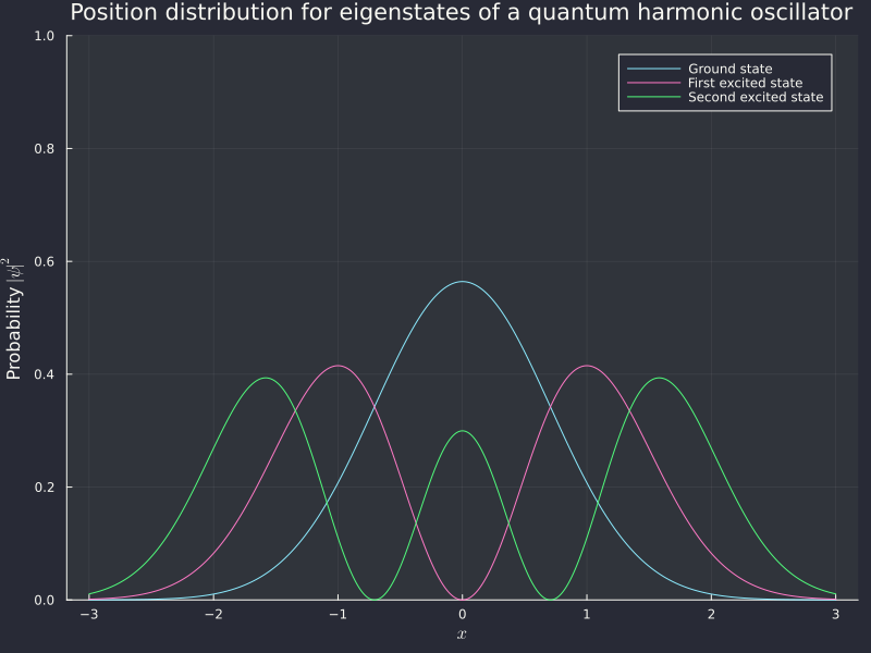
Don't overthink the numbers in these graphs. I used entirely non-physical values for , , and , so the numbers here are not very meaningful. This is called nondimensionalization and it's useful because it lets you appreciate the shape and behavior of a function without getting bogged down in orders of magnitude and units of measurement.
Now that we actually have our initial states— actually wait, one more problem. You see, eigenstates like these are stationary, which means that they do not change in time, so if we were to evolve these, we'd just get the same thing over and over again (believe me, I tried it for science). In fact, here's proof for :
since for an energy eigenstate and we know . The square modulus is
since for any . So evidently the probability distribution does not change in time.
To make these non-stationary, we can just pick a linear combination of them. For simplicity, I elected to use
Cool, now we just need the propagator and we can get to coding!
Propagator
The propagator formally is . Thankfully, this is solvable for the harmonic oscillator (although I didn't solve it myself). The result is called the Mehler kernel:
It's a pretty lengthy expression that hopefully makes you understand why in general we need computers to solve time-dependence.
Crunching numbers
Now we have everything: the starting state and the propagator. The only thing we need is some code and compute power. As usual, I elected to use the Julia programming language because it's just pleasant to work with for scientific computing (though I wish the VSCode extension actually worked properly). The code is not hard: we literally just need to compute the integral
for a bunch of values of and , then plot them together to make a nice little animation. The code is in the harmonic_oscillator_1d_time.jl file. I'm using the QuadGK module to handle one-dimensional numerical integration. The eigenstate functions and the propagator are just a matter of copying notation into Julia. The actual time evolution function is defined as
function ψ_t(x, t, m, ω, initial_state::Function)
    quadgk(y -> propagator(x, y, t, m, ω) * initial_state(y, m, ω), -Inf, +Inf)[1]
end
where I add an initial_function argument that is itself a function, so I can change the starting state on the fly without needing to rewrite the function. The argument inside of quadgk is just the integrand function followed by the integration bounds -Inf and +Inf. The [1] at the end is because quadgk returns a 2-tuple containing both the result and the estimated error, but we only care about the result[5]. To make the animation, the Plots module has a built-in @gif macro to handle that for us. We just make the loop
@time @gif for (i, t) in enumerate(0:0.1:period(ω))
    println("Calculating time $t...")
    if i == 1
        state = initial_state.(x, m, ω)
    else
        state = ψ_t.(x, t, m, ω, initial_state)
    end
    yreal = real(state)
    yimag = imag(state)
    yt = abs2.(state)

    t = round(t, digits=2)
    plot(
        x,
        [[yreal yt], yimag],
        ylims=[(-1, 1) (0, 1)],
        label=[["Real part" L"\frac{\psi_{0}+\psi_{1}}{\sqrt{2}}"] "Imaginary part"],
        xlabel=L"x",
        ylabel=["Probability amplitude" L"Probability $|\psi(x,t)|^2$"],
        title=L"Time evolution of a quantum harmonic oscillator state ($t=%$t$)",
        size=(900, 1200),
        layout=(2, 1),
    )
end fps = 30
Running the code gets us the following graph
Unsupported asset
It works! Sidenote: sorry for the discontinuity in the real and imaginary parts above. The Julia sqrt function has a branch cut over negative reals when given a complex argument, so when the sine in the square root goes over , it jumps because of the cut. I couldn't figure out a way to make it smooth, so I guess it's staying.
So that's it for the harmonic oscillator. Let's move on to the more complicated free particle.
Free particle
Oh free particle. You were so easy in classical mechanics. How the mighty have fallen. The issue here is that the wavefunction of the free particle is not normalizable. As such, it simply has no states that are, at least without further care, physically possible. It has no bound states, like the oscillator above, so the best we can do is state that it exists somewhere, probably, and maybe give a general idea of where in the universe it might be. For this reason, the hunt for the initial state is a bit weird, in that we... don't really have an eigenstates to use like before, so we'll have to figure something out.
Initial state
Sure, maybe there are no energy eigenstates, but there is one thing we can do. See, though the free particle may not have any defined energy value at any given time, clearly must have energy. We can't say how much with certainty, but it's got to have some. So the thing we can do is determine a wave packet. Remember that in quantum mechanics, everything is both a particle and a wave at the same time, so while we can't really look at a point in space and say "there is a particle right there", we can look at a region in space and say "the wave is, for the most part, there". That's, in principle, what a wave packet allows us to do[6]. It allows us to localize a particle within a certain region of space. In a way, it's an exploitation of the uncertainty principle: if we give up our understanding of over time, we can reduce the uncertainty on and give a confidence range for the position. This is what happens when we take a measurement of the position and collapse the wavefunction. We know where it is but not how it moves, until it spontaneously balances out and we lose precision on the position again. That's what we're trying to check here.
As for formulas, the best we can do is express the position starting state as a function of the momentum starting state through a Fourier transform
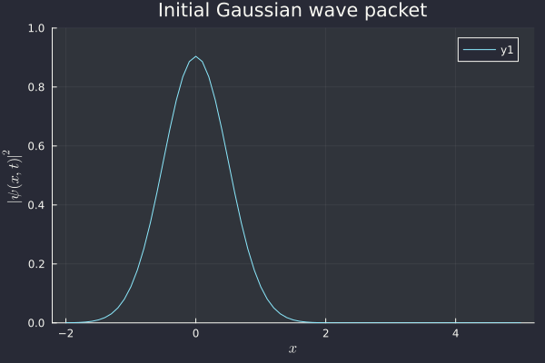
but we can't actually calculate these without the other. There are no "stable" starting states like there are for the harmonic oscillator. As such, we'll just have to pick something arbitrarily and see how that works. The only requirement is that, since these have to obey Fourier transforms, they have to be normalizable (i.e. in ). We care about position, so let's define as the Gaussian wave packet
(I'm being a bit loose with and here, but they're both the same. I'm using because that's the integration variable). The root is the normalization constant. What matters here is the second exponential. It contains , which is a constant, well-defined momentum for the particle. If the Heisenberg inequality is to be believed, a well-defined momentum means that the error on our position should become massive. We'll see. By the way, the nice part about a Gaussian wave packet is that it saturates the Heisenberg inequality, so it gives us the minimum possible uncertainty.
Propagator
Unlike the harmonic oscillator, I have calculated the free particle propagator. However, it's a somewhat ugly-looking derivation, so I'll spare you the details. The propagator is
A bit more compact than the oscillator one.
Crunching numbers
The framework is here basically the same as the oscillator. Define functions of the propagator and initial state, throw them in a numerical integration function and do so for many times and many positions. The code is from free_particle_1d.jl.
function ψ_t(x, t, m, p0)
    quadgk(y -> propagator(x, y, t, m) * ψ_0(y, p0), -Inf, +Inf, rtol=0.0001)[1]
end
y_vals = []
alphas = []
@time @gif for (i, t) in enumerate(0:0.05:4)
    println("Calculating time $t...")
    if i == 1
        init_state = norm.(ψ_0.(x, p_0)) .^ 2
        push!(y_vals, init_state)
        alphas = [1]'
    else
        new_state = @. norm(ψ_t(x, t, m, p_0))^2
        push!(y_vals, new_state)
        alphas = make_alphas(i, decay=0.2)'
    end

    plot(
        x,
        y_vals,
        legend=false,
        alpha=alphas,
        xlims=(-2, 5),
        ylims=(0, 1),
        xlabel=L"x",
        ylabel=L"|\psi(x,t)|^2",
        color=:cyan,
        title=L"Free particle position distribution at time $t=%$t$",
    )
end fps = 12
The alphas that you see here are just to create a fun dissolving effect in the animation. It's just for show.
Unsupported asset
Success! We see an initial peak, but it very quickly disperses as we are unable to know both position and momentum at the same time. Since we know momentum perfectly (), the uncertainty on position is eventually going to shoot up to infinity, which is what we're seeing here. The distribution flattens out and everywhere in the (one-dimensional) universe becomes an equally likely place to find the particle. Inconvenient, but correct.
2D
Before I end this off, I wanted to take do something a bit more visually impactful. Two dimensional plots are fun and all, but 3D plots are much more fun, so let's redo the same thing for a 2D free particle.
The extension is not hard. The initial state can be extended pretty easily by changing scalars into vectors and then renormalizing:
The propagator in dimensions is just the product of one-dimensional propagators
So in 2 dimensions
Throw this in code (in free_particle_2d.jl), evaluate on a grid instead of on a line using HCubature for 2-dimensional numerical integration, plot it in 3D and we get...
Unsupported asset
Conclusion
And that's all. There's a lot more that can be explored here of course, like two-dimensional harmonic oscillators, comparisons between different free particle starting states, different linear combinations of oscillator eigenstates, the hydrogen atom... really, you can do this for any system, though the amount of things that you can figure out analytically gets progressively lower and lower as you stray from the few known systems. I should also probably look into actually optimizing the code: right now, it's just a 1-to-1 replica of the formulas, which is why plotting the 3D animation above took a solid 4 minutes. Maybe I'll use it as an excuse to compare different integration algorithms by implementing them manually. But that's a project for another day.
In the interest of fairness, I'm anthropomorphizing the Universe here as if it had a consciousness and existed solely to spite you. While it may feel like that sometimes, saying "it won't let you" implicitly makes it sound like the "truth" exists out there and we just can't reach it. As far as we can tell, that's false. It's not that we're missing pieces (some "hidden variables", as Einstein called them), the information that we seek is just not there. It's not that we can't tell if a particle is here or there, it simply isn't. It's nowhere, period. The very concept of position falls apart at quantum scales. The only things we can realistically do are: a) accept that that just how it is and b) measure things, as measurements momentarily quell the uncertainty for one or more quantities (so-called wavefunction collapse). ↩
To be fair, so did Heisenberg, as the Heisenberg equation solves time evolution in the Heisenberg picture. ↩
If you've never seen the weird arrow/bracket symbol around the before, that's called a ket and is a part of braket notation (also called Dirac notation). It represent a member of the Hilbert space in which the state is defined. For finite dimensions, it's a row vector. For infinite dimensions, it gets kind of weird, but it usually ends up being a function. ↩
The bra is the flip-side of the ket. If the ket is a row vector, the bra is a column vector. Note that the components of a bra are all complex conjugates. The notation is a scalar/dot product. You might have seen it before as or . ↩
Julia is indexed starting from 1, unlike most programming languages which start at 0. ↩
In practice, wave packets allows us to express an otherwise non-normalizable state as functions that are normalizable. ↩