Simulating Heat

In search for a fancy background for this website's front page, I ended up introducing an entire real-time user-driven heat diffusion simulation running right in your browser.

This website is called Liminal Theater, but I did not feel like there was enough "theater" here. Don't get me wrong, it's colorful and the design choices I made certainly (and voluntarily) aren't quiet and "professional" (whatever that means), but it lacked a certain degree of dynamism. I've always meant for the front page to have a fancy background of sorts, but I never quite knew what to add.

Eventually, revelation struck: what if I made a real-time animated background? Something with physics, or at least something to give me an excuse to solve PDEs in a browser. Thinking and thinking, I envisioned something simple, a minimal simulation that would run based on the user's mouse position that wouldn't tank the browser's performance and eat up a bunch of battery life. Heat diffusion seemed perfect: the heat equation is about as simple as it gets for PDEs in actual use, it's not stiff or pathological in any way, it's an intuitive phenomenon that everyone understands and it can surely be made to look pretty with some creativity. That's it! That was the solution. So I got to work.

Learning to draw

After opening up Liminal Theater's code (a SvelteKit + TypeScript project, if you're curious), I immediately hit the first roadblock: how do I draw stuff on screen? I mean, I knew how to use HTML elements with CSS, but those weren't the solution for a physics sim. I needed the actual screen pixels. A quick search told me that the modern canonical solution for arbitrary graphics rendering in the browser is the Canvas API. So, I set out for the Mozilla Developer Network to read the Canvas API tutorial.

In brief, the Canvas API lets you create a <canvas> element and use its JavaScript API to programmatically draw shapes and paths or render images. If need be, you can access the raw pixel array and draw manually.

To start, I created a <canvas id="simulation"></canvas> element in the front page that will accompany us for the entire rest of this article. I made sure to give it absolute positioning so that it would cover the entire screen without worrying about relative elements, and a negative Z-index so that it would be rendered beneath sibling elements. This set up the basic sandbox for all the graphical things.

At this point, I already knew that space will soon have to be partitioned in cells (more on this later), so my first test was to draw a grid of 10x10 pixel squares, each filled with a random color. The result was this fun glitch-looking screen.

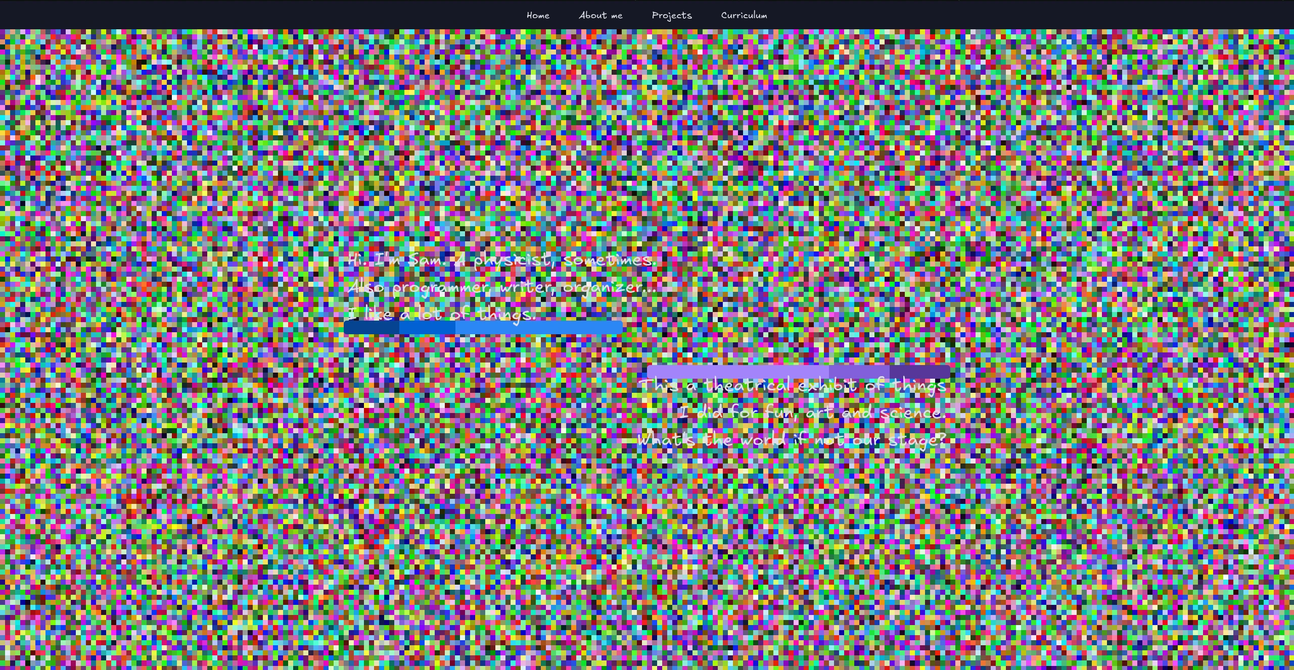
And this was code that made it.^[1]

// Get main page element
const main = document.getElementById('main')!
const width = main.clientWidth
const height = main.clientHeight

// Calculate number of cells at 10x10 px each
const cellWidth = 10
const cellHeight = 10
const horiCells = Math.ceil(width / 10)
const vertCells = Math.ceil(height / 10)

// Set the canvas dimensions to the entire main background
const canvas = document.getElementById('simulation') as HTMLCanvasElement
canvas.width = width
canvas.height = height

// Draw the cells with random colors
const ctx = canvas.getContext('2d')!
for (let i = 0; i < horiCells; i++) {
	for (let j = 0; j < vertCells; j++) {
		const r = Math.random() * 255
		const g = Math.random() * 255
		const b = Math.random() * 255
		ctx.fillStyle = `rgb(${r} ${g} ${b})`
		ctx.fillRect(cellWidth * i, cellHeight * j, cellWidth, cellHeight)
	}
}

Adding interaction

Now that a functioning, if bare bones, canvas and rendering pipeline was set up, the next step was to add some movement. The actual simulation had to wait a little longer because I wanted it to respond to the user's mouse input. Therefore, I added a trackMouse function that fired on mousemove events. On initialization:

document.addEventListener('mousemove', trackMouse)
// Remember to call this on teardown
// document.removeEventListener('mousemove', trackMouse)

Whereas the rendering logic was:

const COLOR_HOT = 'rgb(255 51 0)'
const CELL_WIDTH = 10
const CELL_HEIGHT = 10

function trackMouse(e: MouseEvent) {
	// Find the cell the mouse is currently in
	// The coordinates are in the frame of reference of <main>
	// with the origin being the bounding rect (x,y) of <main>
	const main = document.getElementById('main')!
	const mainOrigin = main.getBoundingClientRect()

	const mouseX = e.clientX - mainOrigin.x
	const mouseY = e.clientY - mainOrigin.y
	const i = Math.floor(mouseX / CELL_WIDTH)
	const j = Math.floor(mouseY / CELL_HEIGHT)

	// Draw that cell with a different color to track the mouse
	const canvas = document.getElementById('simulation') as HTMLCanvasElement
	const ctx = canvas.getContext('2d')!
	ctx.fillStyle = COLOR_HOT
	ctx.fillRect(CELL_WIDTH * i, CELL_HEIGHT * j, CELL_WIDTH, CELL_HEIGHT)
}

This created a very simple system that marked all cells the mouse moved through in red (rgb(255 51 0)).

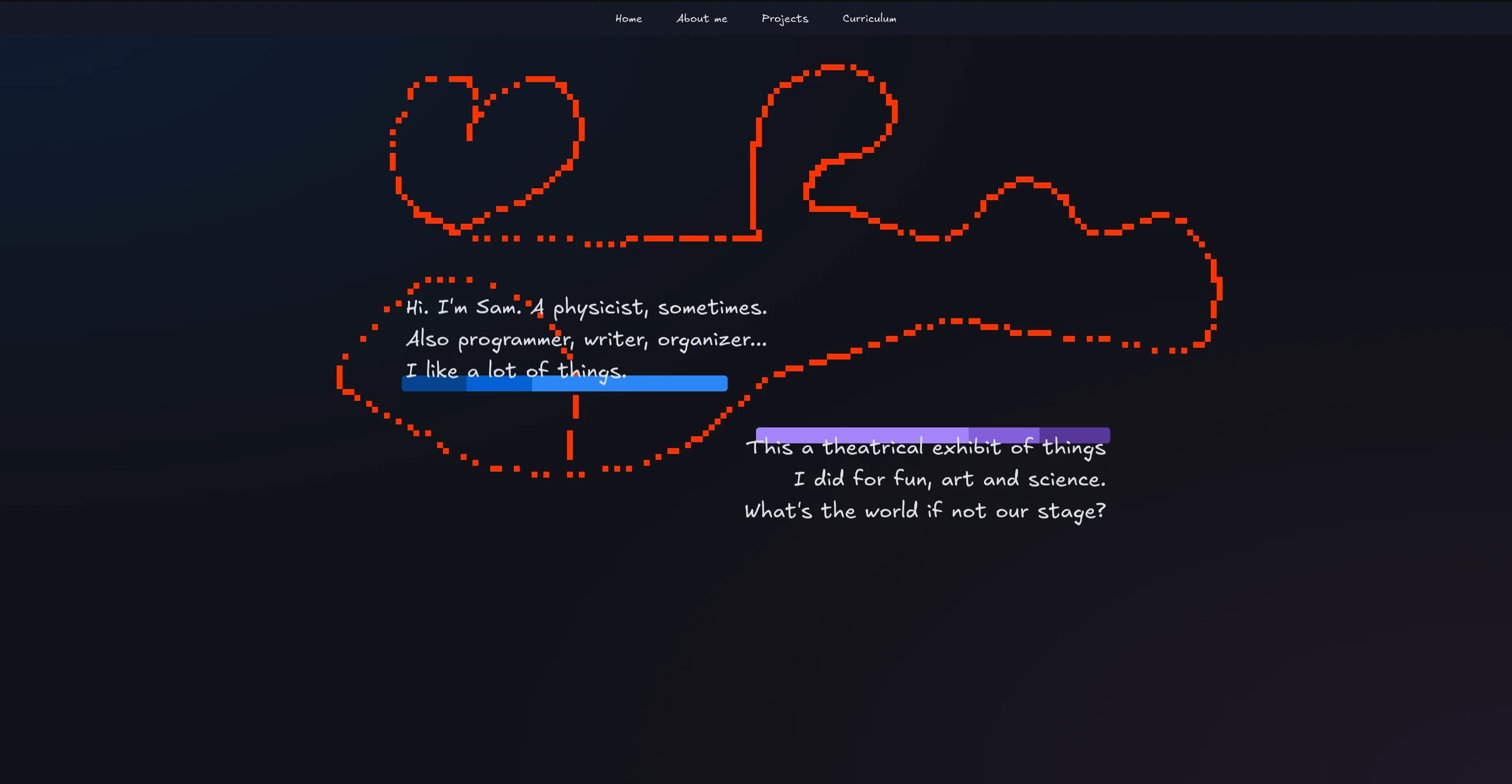
Of course, once drawn, the colored cells remain there forever. With mouse tracking implemented, it was time to add the actual heat diffusion.

Adding a time stepper

The two-dimensional heat equation is this pleasant piece of mathematics:

where $T\equiv T(x,y,t)$ is temperature in a given place $(x,y)$ at a given time $t$. We'll expand on this later, but for now what you need to know is that to solve a PDE on a computer (read: numerically), we need two things: discretization and an integration solver. We'll get to the solver later; for now, let's finish discretization.

Computers don't understand the concept of continuity. They are fundamentally discrete objects (computer memory is, at the end of the day, just long array of bits), so to solve continuous equations numerically, we need to make them discrete too. The heat equation involves both space and time, so we'll need ways to discretize both.

As for space, I've already set up the solution by drawing a grid of identical cells. This is a pretty normal and simple way of doing it, because it's easy to implement and to reason about. Doing it like this, we can (approximately!) solve the equation by only calculating values on (a representative point in) the cells instead of all (infinite) points in $\mathbb{R}^{2}$. Instead of a continuous surface of $T$, we get a matrix of representative values of $T$. If you need the surface, you can interpolate between the representative values, but we won't need that here.

As for time, it works similarly. We need to partition space into discrete amounts of time; time steps, so to speak. In other words, we need to choose at which times $t$ we'll evaluate the equation, just like we choose the cell points $(x,y)$ in space. There are many ways of doing it, but the simplest one is to choose a constant interval of time $\Delta t$ and evaluate once every $\Delta t$. This gives a uniform sequence of evaluations over time; very easy to implement.^[2]

Unlike most scientific simulations, ours will run in real time, so we'll need to make a time stepper that runs in the background. Thankfully, since JavaScript here runs in a persistent real-time environment (the browser), it's pretty easy.

const STEPTIME = 33 // ms (30 FPS)
let timestepperId: number | null = null
function step() {
	// Simulation will go here...
}

// During initialization
timestepperId = setInterval(step, STEPTIME)

// During teardown
clearInterval(timestepperId)
timestepperId = null

The setInterval(fn, period) built-in function creates an infinite asynchronous loop that calls the function fn every period milliseconds. It returns an integer identifier for the loop. The clearInterval(id) cancels the loop of the given id.

In this case, the step function will contain all of the physics calculations that must be done every $\Delta t$, represented by STEPTIME.

Adding heat injection

Before getting to the solver, I tested if this all worked by adding some basic heating. Temperature will be represent visually by a color going from transparent blue (cold) to opaque red (hot). Since we'll be dealing with colors, I made a small utility class for them:

export class CssColor {
	r: number
	g: number
	b: number
	/** Alpha must be [0, 1] not [0%, 100%] */
	alpha: number

	constructor(r: number, g: number, b: number, alpha: number = 1) {
		this.r = r
		this.g = g
		this.b = b
		this.alpha = alpha
	}

	// Returns a CSS color string
	toString() {
		return `rgb(${this.r} ${this.g} ${this.b} / ${this.alpha})`
	}

	// Stands for "linear interpolation"
	lerp(other: CssColor, amount: number) {
		return new CssColor(
			this.r * amount + other.r * (1 - amount),
			this.g * amount + other.g * (1 - amount),
			this.b * amount + other.b * (1 - amount),
			this.alpha * amount + other.alpha * (1 - amount)
		)
	}
}

// During initialization
const COLOR_COLD = new CssColor(0, 51, 102, 0)
const COLOR_HOT = new CssColor(255, 51, 0)

My idea is that the mouse cursor is a hot laser pointer that heats up anything it points to. This is where the real time user input comes from. To implement this, we modify the trackMouse function to only provide the current active cell. The heating logic belongs to step. We don't yet have a way to track temperature, so step just changes the color of the cell, tracked by the CELL_COLORS matrix. We'll replace this matrix later, so don't worry too much about it.

let activeCell: { i: number; j: number } | null = null
function trackMouse(e: MouseEvent) {
	// Find the cell the mouse is currently in
	// The coordinates are in the frame of reference of <main>
	// with the origin being the bounding rect (x,y) of <main>
	const main = document.getElementById('main')!
	const mainOrigin = main.getBoundingClientRect()

	const mouseX = e.clientX - mainOrigin.x
	const mouseY = e.clientY - mainOrigin.y
	const i = Math.floor(mouseX / CELL_WIDTH)
	const j = Math.floor(mouseY / CELL_HEIGHT)

	if (i < 0 || j < 0 || i >= CELL_COLORS.length || j >= CELL_COLORS[0].length) {
		// Check if the indexes are in bounds
		activeCell = null
	} else {
		activeCell = { i, j }
	}
}

function step() {
	if (activeCell) {
		const activeColor = CELL_COLORS[activeCell.i][activeCell.j]

		// The process of heating up is just making the color go from COLD to HOT
		const newColor = activeColor.lerp(COLOR_HOT, 0.99)
		CELL_COLORS[activeCell.i][activeCell.j] = newColor

		// Draw that cell with a different color to track the mouse
		const canvas = document.getElementById('simulation') as HTMLCanvasElement
		const ctx = canvas.getContext('2d')!
		ctx.fillStyle = newColor.toString()
		ctx.fillRect(CELL_WIDTH * activeCell.i, CELL_HEIGHT * activeCell.j, CELL_WIDTH, CELL_HEIGHT)
	}

	timestepperId = setTimeout(step, STEPTIME)
}

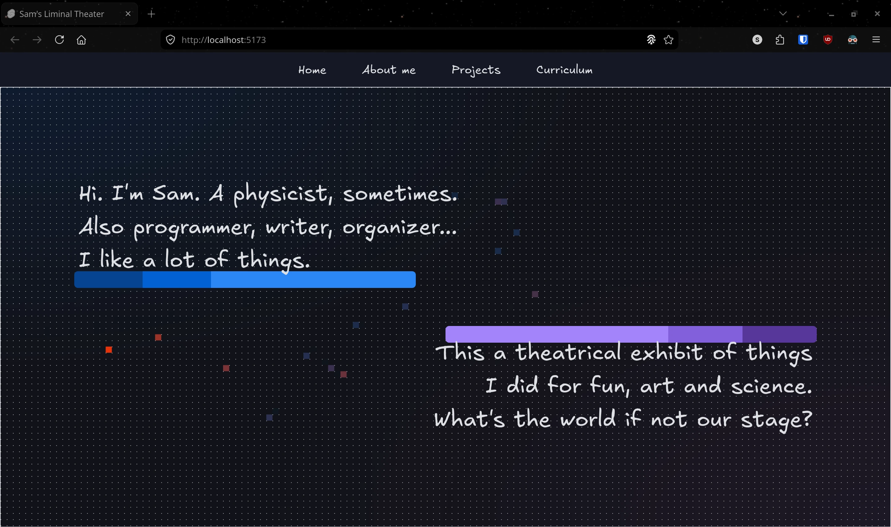
Each step, we push the current cell's color a bit towards red and draw it. There's no diffusion or cooling yet, so the heating is permanent. The result looks like this:

For clarity, I also added dots to show the grid.

// During canvas initialization
const canvas = document.getElementById('simulation')! as HTMLCanvasElement
const ctx = canvas.getContext('2d')!
const parentDims = canvas.parentElement!.getBoundingClientRect()
const dpr = window.devicePixelRatio

// Set DPR-aware sizes
canvas.width = parentDims.width * dpr
canvas.height = parentDims.height * dpr
ctx.scale(dpr, dpr)
canvas.style.width = `${Math.floor(parentDims.width)}px`
canvas.style.height = `${Math.floor(parentDims.height)}px`

Solving the heat equation

After all of this preparation, we can finally start tackling the heat equation itself. The heat equation is a second-order partial differential equation of the form

$T(x,y,t)\equiv T$ is the temperature at point $(x,y)$ and time $t$.^[3] The Newton dot notation indicates the time derivative: $\dot{T}\equiv \frac{ \partial T }{ \partial t }$. The Laplacian operator indicates the sum of all spatial second derivatives. We are working in two dimensions, so the form we get is

Like all differential equations, it's continuous, so we need to turn it into something that works on a discrete grid over discrete time steps. Here, I used central finite differences to discretize space. The idea behind finite differences is to take the definition of derivative and approximate the limit with a finite difference:

where we take $\Delta x$ to be small but not infinitesimal. Because the limit is gone, this expression no longer requires a continuous space. We hence reinterpret $\Delta x$ to be the grid spacing, assuming identical cells of size $\Delta x\times \Delta y$. Call $x_{i}$ the $x$ coordinate of the cell $(i,j)$. Then, the finite difference on $x$ between cells $(i,j)$ and $(i+1,j)$ is

This is a forward difference because it involves an element $i$ and the next one $i+1$. The central difference is the same, but shifted by half a cell size so that it is centered on just $i$, without needing the next one:

(There's also the backward difference between $i$ and $i-1$.) You can apply this rule to second derivatives too, to get the second-order central difference

We can now apply this to the heat equation. Rename $f(x)$ to $T(x,y,t)$, adapt the above expression to partial derivatives and use the shorthand $T(x_{i},y_{j},t)\equiv T_{i,j}$ to state:

Likewise for the $y$ derivative. For simplicity, let the grid cells be square. Then, $\Delta x=\Delta y=h$ and each cell has size $h\times h$. With this, we have a proper approximation of the right-hand side of $(1)$. Plug $(2)$ into $(1)$ to get

Great! Are we done? No. The time derivative is still continuous. We need to discretize over the time steps too. Specifically, we need to figure out how to go from $T_{i,j}$ at time step $n$ to $T_{i,j}$ at time step $n+1$. Let $T_{i,j}^{n}$ be the value of $T_{i,j}$ at the $n$-th time step. Then, in general, we have

The function $S$ is the time integration scheme, that is, the solver that I mentioned above. It takes the derivative at the current time step and uses it to give a best-effort guess on how $T$ will change in the next $\Delta t$ seconds (or other time units). This scheme replaces the time derivative in the same way as the finite differences replace the space derivatives. With both defined, the problem is well-put and the computer can solve.

How do we choose $S$? Well, there's a lot of options for $S$. The main parameters that we use to discern between one $S$ and another is how accurately it guesses the derivative, how stable it is in when the equation varies rapidly, and how long it takes to run. The big constraint here is that this simulation must run in the background in the user's browser, which may be powerful desktop computer or a jank laptop on battery power. Or worse, a phone. We can't afford this simulation to be expensive to run because otherwise it risks lagging the website, overheat the device and drain battery just due to visiting the front page, which is bad user experience and just plain rude. Thus, I opted for the simplest, least expensive integration scheme: explicit Euler.

Explicit Euler integration is almost trivially easy:

That's it. Just multiply the derivative by the time step. This scheme has lots of problems, not the least of which poor accuracy and bad stability (which surely won't come back to haunt me later, right? Right?), but performance is not one of them, so that's what we'll go with. This simulation's only purpose is to look pretty: who cares if it's a little inaccurate? Plug the above into $(4)$, use $(3)$ and we get our definitive, fully discrete PDE approximation:

This is still the same heat equation as $(1)$, but approximated to discrete space and time. This is something that a computer can indeed understand, so the only step we have left to take is to write this into actual computer code.

Actually no, that's not it, we are not done. (I'm sorry.) A differential equation cannot be fully solved without boundary conditions and initial conditions.

A simulation is kind of like an inductive proof. We start from somewhere, then give a rule on how to step forward. $(5)$ is the step. Initial conditions are the start. In our case, we ask ourselves: what is $T_{i,j}^{0}$ for all $(i,j)$? For simplicity, we'll start with everything frozen at absolute zero. Formally: $T_{i,j}^{0}=0\ \forall\ i,j$. This makes the simulation do nothing until the user injects heat somewhere.

Boundary conditions determine what happens when you hit the edges of the simulation. In our case, what happens at the edges of the grid? There, the indexes $i\pm1$ or $j\pm1$ might be out of bounds. I chose Dirichlet boundary conditions, which here mean that all out-of-bounds cells are treated as being permanently frozen at $T=0$. If you want a physical interpretation, it's like the world around the grid is stuck at absolute zero, so that when heat flows out of the grid (i.e., it goes into an out-of-bounds cell), it is dissipated and lost. Eventually, all heat in the grid will flow out and the grid will stabilize at $T=0$. In technical terms, the environment is a heat reservoir at absolute zero.

Ok, now we are actually done, I promise. We can now start working on the code.

Implementing the solver

I'll spare you the details of how I got to this code. There was some trial and error, a good bit of it actually. It wouldn't be mathematical code if it didn't have inexplicable errors sometimes.

The full code is available at the bottom of this page, so I'm focusing on just the important parts here. If you really need the full context, you can look there.

// During initialization
// Explicit Euler is stable when Delta t/h^2 <= 0.25
// Since h depends on DPR we need to update Delta t too
// We set to 0.1 instead of 0.25 just in case
STEPTIME = 0.1 * CELL_EDGE * CELL_EDGE
// Get window height/width ...
ROWS = Math.ceil(height / CELL_EDGE)
COLS = Math.ceil(width / CELL_EDGE)
TEMP = Array.from({ length: COLS }, () => new Array(ROWS).fill(0))
TEMP_NEXT = Array.from({ length: COLS }, () => new Array(ROWS).fill(0))

This code sets up the simulation quantities and runs right after initializing the canvas. You'll see that STEPTIME (a.k.a. $\Delta t$) is no longer a constant, but rather chosen based on CELL_EDGE (a.k.a. $h$). The issue is that explicit Euler in quite unstable. If $\Delta t$ is too large, the whole simulation goes off the rails with admittedly pretty funny results. See for instance:

A good rule of thumb for stability with explicit Euler is to choose $\Delta t$ such that $\Delta t\leq0.25h^{2}$. I chose $\Delta t=0.1h^{2}$.

ROWS and COLS are variable because the grid fills the entire canvas, but the canvas' size depends on the browser window's size, so we can't know how large the grid is are until the page loads. (Later I'll add dynamic resizing.) The number of rows and columns is found by finding how many cells of size $h\times h$ can fit in the canvas.

TEMP and TEMP_NEXT are two real $\text{ROWS}\times\text{COLS}$ matrices. TEMP holds the current temperature $T_{i,j}^{n}$ for all grid cells, while TEMP_NEXT holds the next step's temperature $T_{i,j}^{n+1}$ that we calculate throughout the step. Never update the state (that is, assign $T_{i,j}^{n+1}$ to $T_{i,j}^{n}$) in the middle of a step! The next step's values must be calculated using the current step. If you overwrite $T_{i,j}^{n}$ with $T_{i,j}^{n+1}$ as you go, you'll end up with mixed calculations where some values are current and some values are next. That breaks the logic of the simulation and leads to hard-to-trace inconsistencies. What you do is store the next step separately and update in bulk only at the very end of the physics step.

function step() {
	const canvas = document.getElementById('simulation') as HTMLCanvasElement
	const ctx = canvas.getContext('2d')!

	// 1. Diffuse heat across all cells
	for (let i = 0; i < COLS; i++) {
		for (let j = 0; j < ROWS; j++) {
			// Dirichlet boundary conditions: treat all out-of-bounds cells
			// as having a permanent temperature of 0
			const T_i_j = TEMP[i][j]
			const T_ip1_j = i + 1 < COLS ? TEMP[i + 1][j] : 0
			const T_im1_j = i - 1 >= 0 ? TEMP[i - 1][j] : 0
			const T_i_jp1 = j + 1 < ROWS ? TEMP[i][j + 1] : 0
			const T_i_jm1 = j - 1 >= 0 ? TEMP[i][j - 1] : 0

			// Explicit Euler integration
			const delta =
				(STEPTIME / (CELL_EDGE * CELL_EDGE)) *
				(T_ip1_j + T_im1_j + T_i_jp1 + T_i_jm1 - 4 * T_i_j)
			TEMP_NEXT[i][j] = TEMP[i][j] + delta

			// Clamp temperature to the valid range of [0, 1]
			if (TEMP_NEXT[i][j] < 0) TEMP_NEXT[i][j] = 0
			if (TEMP_NEXT[i][j] > 1) TEMP_NEXT[i][j] = 1
		}
	}

	// 2. If the mouse is hovering over a cell, inject heat
	if (activeCell) {
		let activeHeat = TEMP_NEXT[activeCell.i][activeCell.j]
		TEMP_NEXT[activeCell.i][activeCell.j] = Math.min(1.0, activeHeat + 0.2)
	}

	// 3. Update old temperature with the new one
	TEMP = TEMP_NEXT

	// 4. Update visual cell color
	ctx.clearRect(0, 0, canvas.width, canvas.height)
	for (let i = 0; i < COLS; i++) {
		for (let j = 0; j < ROWS; j++) {
			ctx.fillStyle = COLOR_COLD.lerp(COLOR_HOT, TEMP[i][j]).toString()
			ctx.fillRect(CELL_EDGE * i, CELL_EDGE * j, CELL_EDGE, CELL_EDGE)
		}
	}
}

There's four substeps going on here.

The first is heat diffusion. This is where we run explicit Euler. delta is $S(\dot{T}_{i,j}^{n})$ and the update of TEMP_NEXT[i][j] is $(5)$. The Dirichlet boundary conditions are implemented as ternary operators when reading temperatures. Finally, I chose the temperature to be bounded between 0 and 1. The lower bound is physical (absolute zero), while the upper bound is just a convenience. In the real world, temperature can be arbitrarily high,^[4] but here I capped it to 1 just so I could interpret $T$ as a percentage and use it as the interpolation value for CssColor.lerp. When $T_{i,j}^{n}=0$, the corresponding grid cell $(i,j)$ is COLOR_COLD, when $T_{i,j}^{n}=1$ the cell is COLOR_HOT, when it's in between, it's a linear mix of the two colors. Plain and simple.

The second substep is injecting heat. It's the same as before, just updated to the new logic. I add a constant 0.2 to a cell's $T$ every step the mouse cursor is hovering over that cell, up to $T=1$.

The third substep is applying the temperature changes by overwriting TEMP with TEMP_NEXT. At this point, the physics is all done.

The fourth substep is the graphical part. For each cell, color it to match then new temperature.

With this code, I was done! This is all that's needed for a real time heat diffusion simulation. You can see the result here:

Making it pretty

While it worked, I was a little unsatisfied. It had physics, sure, but it lacked visual flair. Heat dissipates so fast it doesn't really leave much of an afterimage. What if I forced it to?

I added a new matrix MIN_ALPHA that records the alpha (opacity) value that each cell achieves due to interpolation. It starts from zero and is updated each step. The important part is that it is monotonically increasing: each value $\alpha_{i,j}$ cannot decrease. When calculating the new cell color, if it would have an $\alpha_{i,j}$ lower than the recorded minimum, it is replaced by the minimum. In other words, it can never become more transparent ever again.

This has the consequence that whenever a cell is heated up, it is permanently "burned" and will never vanish. It will cool down to a nice cold blue color when $T\to 0$, but it won't become transparent. This creates persistent trails that mark all the places that were heated and how much they were heated, leading to the very afterimages I alluded to before.

Making it better

With a satisfying simulation in hand, I added some finishing touches. I won't bore you with the technicalities. Briefly:

• Skip cells that are below $T_\text{min}$ with all surrounding cells also at $T_\text{min}$, with $T_\text{min}= 10^{-10}$. This avoids computing $S(\dot{T}^{n}_{i,j})$ for cells at (almost) absolute zero.
• Skip draw calls for cells with $\alpha_{i,j}<0.001$. This avoids drawing invisible cells.
• Move drawing logic (third subset) to window.requestAnimationFrame(fn) calls. This is a browser built-in function that schedules a function fn to run when the browser renders graphics. It helps to decouple the render loop from the physics loops, which is best practice.
• Reset the grid every time the user resizes the browser window. The grid size depends on the window size, so it needs to be responsive to UI updates.
• Limit the number of columns that a grid can have to avoid huge grids on large screens, which can be very compute-heavy.
• Add touchscreen tracking on top of mouse cursor tracking so that the page works on mobile devices too.

The final version of the code is freely available at the bottom of the page.

Conclusion

I'll be honest, I thought JavaScript would be a much worse language to implement a physics simulation in. It actually wasn't that bad! For isolated simulations like this, it worked quite nicely. I wouldn't use it for anything scientific, though. The actual difficult (and interesting) part of this project was the interactive visualization, which was the real goal of the project anyway. I think it came out quite nicely! Getting to mix physics, scientific computing, web development and graphics programming was an odd and certainly very niche experience, but it goes to show that there's a lot of value to be had in playing matchmaker between foreign disciplines.

There's a whole lot that can be improved. Physics-wise, I could try periodic boundary conditions, add a heat diffusivity term and/or a cooling term to the heat equation. More likely though, it would be better to improve the UX and add a modal or drawer dashboard on the home page that can be used to change the parameters of the simulation on the fly, as well as disable it entirely. That way, I can also add different kinds of simulations and pick one at random each time the front page loads, or let the user choose their favorite. There's also a possible parallelization approach, maybe with Web Workers, but it's difficult to add in a browser due to threads being already populated internally by the browser. Oh well, more food for thought.

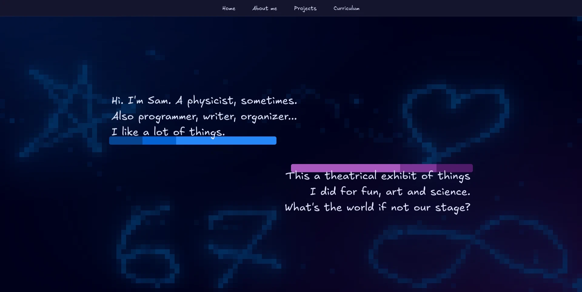
I'll leave this off with a silly creation I made with the heat trails. Until next time!

All of the code

This simulation is implemented as a Svelte component. Save this code as HeatDiffusion.svelte (or some other name), then import it and add it as <HeatDiffusion /> wherever you want. It should inherit the dimensions of the parent element.

If you don't use Svelte, you can extract the code in the <script> tag, manually add the <canvas> somewhere else and do the initialization wherever you prefer.

<!--
MIT License

Copyright (c) 2026 Samuele Vignoli

Permission is hereby granted, free of charge, to any person obtaining a copy
of this software and associated documentation files (the "Software"), to deal
in the Software without restriction, including without limitation the rights
to use, copy, modify, merge, publish, distribute, sublicense, and/or sell
copies of the Software, and to permit persons to whom the Software is
furnished to do so, subject to the following conditions:

The above copyright notice and this permission notice shall be included in all
copies or substantial portions of the Software.

THE SOFTWARE IS PROVIDED "AS IS", WITHOUT WARRANTY OF ANY KIND, EXPRESS OR
IMPLIED, INCLUDING BUT NOT LIMITED TO THE WARRANTIES OF MERCHANTABILITY,
FITNESS FOR A PARTICULAR PURPOSE AND NONINFRINGEMENT. IN NO EVENT SHALL THE
AUTHORS OR COPYRIGHT HOLDERS BE LIABLE FOR ANY CLAIM, DAMAGES OR OTHER
LIABILITY, WHETHER IN AN ACTION OF CONTRACT, TORT OR OTHERWISE, ARISING FROM,
OUT OF OR IN CONNECTION WITH THE SOFTWARE OR THE USE OR OTHER DEALINGS IN THE
SOFTWARE.
-->

<script lang="ts">
	import { browser } from '$app/environment'
	import { CssColor } from '$lib/utils'
	import { onMount } from 'svelte'

	const canvasId = 'simulation'

	const COLOR_COLD = new CssColor(0, 51, 102, 0)
	const COLOR_HOT = new CssColor(255, 51, 0)

	const CELL_EDGE_BASE = 10
	let CELL_EDGE = CELL_EDGE_BASE
	let ROWS = 0
	let COLS = 0
	const MAX_COLS = 120

	let STEPTIME = 33 // ms

	/** Outer array is columns (x/i), inner arrays are rows (y/j). */
	let TEMP: number[][] = [[]]
	let TEMP_NEXT: number[][] = [[]]
	let MIN_ALPHA: number[][] = [[]]

	let activeCell: { i: number; j: number } | null = null
	let timestepperId: number | null = null
	let resizeDebounceId: number | null = null

	function setActiveCell(x: number, y: number) {
		// Find the cell the given coords are currently in
		// The coordinates are in the frame of reference of the parent
		// with the origin being the bounding rect (x,y) of the parent
		const parent = document.getElementById(canvasId)!.parentElement!
		const origin = parent.getBoundingClientRect()
		const shiftedX = x - origin.x
		const shiftedY = y - origin.y
		const i = Math.floor(shiftedX / CELL_EDGE)
		const j = Math.floor(shiftedY / CELL_EDGE)
		if (i < 0 || j < 0 || i >= COLS || j >= ROWS) {
			// Check if the indexes are in bounds
			activeCell = null
		} else {
			activeCell = { i, j }
		}
	}

	function trackMouse(e: MouseEvent) {
		setActiveCell(e.clientX, e.clientY)
	}

	function trackTouch(e: TouchEvent) {
		e.preventDefault()
		setActiveCell(e.touches[0].clientX, e.touches[0].clientY)
	}

	function onMouseOut(_: MouseEvent) {
		activeCell = null
	}

	function fitCanvas() {
		const canvas = document.getElementById(canvasId)! as HTMLCanvasElement
		const ctx = canvas.getContext('2d')!
		const parentDims = canvas.parentElement!.getBoundingClientRect()
		const dpr = window.devicePixelRatio

		// Set DPR-aware sizes
		canvas.width = parentDims.width * dpr
		canvas.height = parentDims.height * dpr
		ctx.scale(dpr, dpr)
		canvas.style.width = `${Math.floor(parentDims.width)}px`
		canvas.style.height = `${Math.floor(parentDims.height)}px`

		// To avoid massive grids, we cap the horizontal cell count
		const minCellEdge = Math.ceil(canvas.width / MAX_COLS)
		CELL_EDGE = Math.max(minCellEdge, CELL_EDGE_BASE * dpr)
		// Explicit Euler is stable when Delta t/h^2 <= 0.25
		// Since h depends on DPR we need to update Delta t too
		// We set to 0.1 instead of 0.25 just in case
		STEPTIME = 0.1 * CELL_EDGE * CELL_EDGE

		// Reset the grid to match the canvas
		ROWS = Math.ceil(canvas.height / CELL_EDGE)
		COLS = Math.ceil(canvas.width / CELL_EDGE)
		TEMP = Array.from({ length: COLS }, () => new Array(ROWS).fill(0))
		TEMP_NEXT = Array.from({ length: COLS }, () => new Array(ROWS).fill(0))
		MIN_ALPHA = Array.from({ length: COLS }, () => new Array(ROWS).fill(0))
	}

	function fitCanvasDebounced(_: Event) {
		if (resizeDebounceId) clearTimeout(resizeDebounceId)
		resizeDebounceId = setTimeout(fitCanvas, 300)
	}

	function step() {
		// Diffuse heat across all cells
		for (let i = 0; i < COLS; i++) {
			for (let j = 0; j < ROWS; j++) {
				// Dirichlet boundary conditions: treat all out-of-bounds cells
				// as having a permanent temperature of 0
				const T_i_j = TEMP[i][j]
				const T_ip1_j = i + 1 < COLS ? TEMP[i + 1][j] : 0
				const T_im1_j = i - 1 >= 0 ? TEMP[i - 1][j] : 0
				const T_i_jp1 = j + 1 < ROWS ? TEMP[i][j + 1] : 0
				const T_i_jm1 = j - 1 >= 0 ? TEMP[i][j - 1] : 0

				// For performance, skip frozen regions (T~0 for cell and neighbors)
				const min = 1e-10
				if (T_i_j < min && T_ip1_j < min && T_im1_j < min && T_i_jp1 < min && T_i_jm1 < min)
					continue

				// We use explicit Euler as the integration scheme for performance reasons
				const delta =
					(STEPTIME / (CELL_EDGE * CELL_EDGE)) *
					(T_ip1_j + T_im1_j + T_i_jp1 + T_i_jm1 - 4 * T_i_j)
				TEMP_NEXT[i][j] = TEMP[i][j] + delta

				// Clamp temperature to the valid range of [0, 1]
				if (TEMP_NEXT[i][j] < 0) TEMP_NEXT[i][j] = 0
				if (TEMP_NEXT[i][j] > 1) TEMP_NEXT[i][j] = 1
			}
		}

		// If the mouse is hovering over a cell, inject heat
		if (activeCell) {
			let activeHeat = TEMP_NEXT[activeCell.i][activeCell.j]
			TEMP_NEXT[activeCell.i][activeCell.j] = Math.min(1.0, activeHeat + 0.2)
		}

		// Update temperature
		TEMP = TEMP_NEXT

		// Draw the grid. Instead of forcing the draw, we request it to the
		// browser, which will issue it when ready. Helps decouple physics
		// framerate from graphical framerate
		window.requestAnimationFrame(drawGrid)
	}

	function drawGrid() {
		const canvas = document.getElementById(canvasId) as HTMLCanvasElement
		const ctx = canvas.getContext('2d')!

		ctx.clearRect(0, 0, canvas.width, canvas.height)
		for (let i = 0; i < COLS; i++) {
			for (let j = 0; j < ROWS; j++) {
				const newColor = COLOR_COLD.lerp(COLOR_HOT, TEMP[i][j])

				// Alpha is monotonically increasing, like the screen's getting burned
				// This creates permanent "remnants" after adding heat
				if (newColor.alpha > MIN_ALPHA[i][j]) {
					MIN_ALPHA[i][j] = newColor.alpha
				} else {
					newColor.alpha = MIN_ALPHA[i][j]
				}

				// For performance, we avoid draw calls for any cell that
				// would be basically invisible to the human eye
				if (newColor.alpha < 0.001) continue

				ctx.fillStyle = newColor.toString()
				ctx.fillRect(CELL_EDGE * i, CELL_EDGE * j, CELL_EDGE, CELL_EDGE)
			}
		}
	}

	onMount(() => {
		if (browser) {
			// Set the initial state of the canvas and grid
			fitCanvas()
			const canvas = document.getElementById(canvasId) as HTMLCanvasElement
			const ctx = canvas.getContext('2d')!
			ctx.fillStyle = COLOR_COLD.toString()
			ctx.fillRect(0, 0, canvas.width, canvas.height)

			// Uncomment this to visualize the grid
			// ctx.fillStyle = 'rgb(200, 200, 200)'
			// for (let i = 0; i < COLS; i++) {
			// 	for (let j = 0; j < ROWS; j++) {
			// 		ctx.fillRect(CELL_EDGE * i, CELL_EDGE * j, 1, 1)
			// 	}
			// }

			// Add the mouse tracker, responsive resizing and start the simulation
			document.addEventListener('mousemove', trackMouse)
			document.addEventListener('touchmove', trackTouch)
			document.addEventListener('mouseout', onMouseOut)
			window.addEventListener('resize', fitCanvasDebounced)
			timestepperId = setInterval(step, STEPTIME)
		}

		return () => {
			// Clean up simulation tools
			document.removeEventListener('mousemove', trackMouse)
			document.removeEventListener('touchmove', trackTouch)
			document.removeEventListener('mouseout', onMouseOut)
			window.removeEventListener('resize', fitCanvas)
			if (timestepperId !== null) {
				clearInterval(timestepperId)
				timestepperId = null
			}
		}
	})
</script>

<canvas id={canvasId} class="absolute -z-10"></canvas>

This is the CssColor implementation. I placed it in a separate utils.ts file, but you can copy it anywhere you prefer.

// MIT License
// Copyright (c) 2026 Samuele Vignoli

export class CssColor {
	r: number
	g: number
	b: number
	/** Alpha must be [0, 1] not [0%, 100%] */
	alpha: number

	constructor(r: number, g: number, b: number, alpha: number = 1) {
		this.r = r
		this.g = g
		this.b = b
		this.alpha = alpha
	}

	toString() {
		return `rgb(${this.r} ${this.g} ${this.b} / ${this.alpha})`
	}

	lerp(other: CssColor, amount: number) {
		return new CssColor(
			this.r * (1 - amount) + other.r * amount,
			this.g * (1 - amount) + other.g * amount,
			this.b * (1 - amount) + other.b * amount,
			this.alpha * (1 - amount) + other.alpha * amount
		)
	}
}